
Case study: an explanatory model of verbal aggression
Source:vignettes/articles/case-study-verbal-aggression.Rmd
case-study-verbal-aggression.RmdThe verbal aggression data contain the responses of 316 students to
24 items (De Boeck and Wilson, 2004; Smits, De Boeck, and Vansteelandt,
2004). Each item combines one of four frustrating situations, one of
three possible responses—cursing, scolding or shouting—and whether the
respondent wants to respond that way or would actually do so. Responses
are no, perhaps and yes, scored
0, 1 and 2.
This crossed item design makes the data useful for illustrating the linear partial credit model (LPCM). Rather than estimate every item threshold freely, the LPCM explains them from the characteristics used to construct the items.
data("VerbalAggression", package = "psychotools")
responses <- VerbalAggression$resp
item_names <- colnames(responses)

item_design <- data.frame(
  item = item_names,
  situation = factor(substr(item_names, 1, 2), levels = paste0("S", 1:4)),
  mode = factor(ifelse(grepl("Want", item_names), "want", "do"),
                levels = c("do", "want")),
  behaviour = factor(
    sub("^S[1-4](Want|Do)", "", item_names),
    levels = c("Curse", "Scold", "Shout")
  )
)

head(item_design)
#>          item situation mode behaviour
#> 1 S1WantCurse        S1 want     Curse
#> 2   S1DoCurse        S1   do     Curse
#> 3 S1WantScold        S1 want     Scold
#> 4   S1DoScold        S1   do     Scold
#> 5 S1WantShout        S1 want     Shout
#> 6   S1DoShout        S1   do     Shout
These are categorical item predictors. Person variables such as gender and anger are not item predictors; they may instead be examined later through targeting or differential item functioning.
An additive model
We begin with additive effects for situation, mode and behaviour. The
reserved threshold factor distinguishes the transition from
no to perhaps from the transition from
perhaps to yes. Its interaction with mode
allows that threshold structure to differ between wanting to act and
actually acting.
fit_additive <- rasch_explanatory(
  responses,
  predictors = item_design,
  formula = ~ situation + mode + behaviour + threshold + mode:threshold
)

explanatory_test(fit_additive)
#>  model parameters free_parameters r_squared r_squared_adj              r2_basis
#>   LPCM          8              47     0.894         0.871 threshold calibration
#>     chisq df p_naive chisq_kent       p  p_kent
#>  1820.943 39 < 0.001    157.719 < 0.001 < 0.001
The Kent-adjusted comparison rejects this restriction (\(\chi^2_{39} = 157.72\), \(p < .001\)). The additive formulation does not capture all systematic differences among the items.
Interactions in the item design
The factorial construction also permits interactions among situation, mode and behaviour. The following model includes every two-way interaction among those characteristics and allows each characteristic to alter the response threshold structure:
fit_explanatory <- rasch_explanatory(
  responses,
  predictors = item_design,
  formula = ~ (situation + mode + behaviour)^2 +
    threshold * (situation + mode + behaviour)
)

model_test <- explanatory_test(fit_explanatory)
model_test
#>  model parameters free_parameters r_squared r_squared_adj              r2_basis
#>   LPCM         24              47     0.976         0.949 threshold calibration
#>    chisq df p_naive chisq_kent     p p_kent
#>  290.552 23 < 0.001     26.295 0.287  0.287
This model estimates 24 explanatory coefficients in place of 47 free threshold parameters. Its Kent-adjusted comparison with the free calibration is not significant (\(\chi^2_{23} = 26.30\), \(p = .287\)). The explanatory structure therefore gives a materially smaller calibration without a detected loss of fit in these data. It reproduces 97.6% of the variation in the free threshold calibration, and 94.9% after adjusting for the twenty-four coefficients doing the reproducing.
The threshold estimates from the explanatory and free calibrations are shown below. Points close to the diagonal indicate where the predictor structure reproduces the freely estimated threshold.
threshold_comparison <- merge(
  fit_explanatory$reference_fit$est$thr[c("item", "k", "tau")],
  fit_explanatory$est$thr[c("item", "k", "tau")],
  by = c("item", "k"),
  suffixes = c("_free", "_explanatory")
)

plot(
  threshold_comparison$tau_free,
  threshold_comparison$tau_explanatory,
  pch = c(1, 19)[threshold_comparison$k],
  xlab = "Free threshold estimate (logits)",
  ylab = "Explanatory threshold estimate (logits)"
)
abline(0, 1, lty = 2, col = "grey40")
legend("topleft", legend = c("First threshold", "Second threshold"),
       pch = c(1, 19), bty = "n")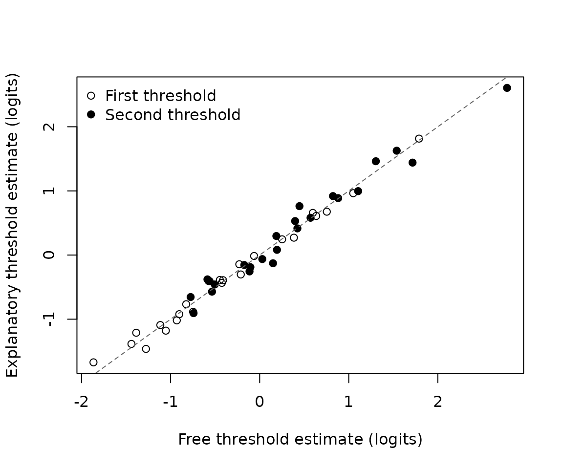
Free and explanatory threshold estimates for the verbal aggression items.
The coefficient table is on the threshold-location scale. A positive
coefficient raises the relevant threshold and makes endorsement less
likely; a negative coefficient makes it more likely. Main effects refer
to the reference levels shown in item_design, and an
interaction modifies the corresponding main effect.
effects <- fit_explanatory$est$coefficients
effects[effects$p_adj < .05,
        c("term", "estimate", "se", "t", "df", "p", "p_adj")]
#>                        term estimate    se      t  df       p   p_adj
#>                 situationS3    0.952 0.121  7.878 309 < 0.001 < 0.001
#>              behaviourScold    0.619 0.109  5.651 309 < 0.001 < 0.001
#>              behaviourShout    1.631 0.130 12.549 309 < 0.001 < 0.001
#>                  threshold2    0.815 0.184  4.423 309 < 0.001 < 0.001
#>        situationS2:modewant   -0.416 0.081 -5.119 309 < 0.001 < 0.001
#>        situationS3:modewant   -0.507 0.104 -4.892 309 < 0.001 < 0.001
#>  situationS3:behaviourScold    0.425 0.106  4.015 309 < 0.001   0.001
#>  situationS4:behaviourScold    0.329 0.098  3.375 309 < 0.001   0.012
#>  situationS3:behaviourShout    0.618 0.134  4.628 309 < 0.001 < 0.001
#>  situationS4:behaviourShout    0.425 0.122  3.487 309 < 0.001   0.008
#>     modewant:behaviourShout   -0.574 0.114 -5.038 309 < 0.001 < 0.001
#>   behaviourShout:threshold2   -0.531 0.175 -3.026 309   0.003   0.035
For example, the positive coefficients for
behaviourScold and behaviourShout indicate
that these responses are harder to endorse than cursing in the reference
situation and mode. Their interactions show where that difference
changes. The threshold interactions describe changes in the distance
between no, perhaps and yes,
rather than changes in the item location as a whole.
Checking fixed departures
The model comparison assesses the explanatory restrictions jointly.
explanatory_diagnostics() then checks whether any single
item-location or threshold-structure departure remains after the active
model has been fitted. Holm adjustment covers the complete set of
candidate departures.
departures <- explanatory_diagnostics(fit_explanatory)
head(departures, 10)
#>         item           component parameters_added departure deviance_reduction
#>  S1WantShout Threshold structure                1     0.320             67.958
#>  S1WantScold Threshold structure                1     0.258             43.595
#>  S2WantCurse Threshold structure                1     0.263             43.002
#>  S4WantShout Threshold structure                1     0.259             35.892
#>    S2DoCurse Threshold structure                1     0.224             33.596
#>  S1WantCurse Threshold structure                1     0.218             30.708
#>  S4WantCurse Threshold structure                1     0.196             26.631
#>  S4WantScold       Item location                1     0.246             19.167
#>    S4DoScold       Item location                1    -0.246             19.167
#>  S3WantCurse Threshold structure                1     0.160             16.779
#>  df     p weak converged p_adj
#>   1 0.030              * 1.000
#>   1 0.045              * 1.000
#>   1 0.042              * 1.000
#>   1 0.110              * 1.000
#>   1 0.112              * 1.000
#>   1 0.105              * 1.000
#>   1 0.123              * 1.000
#>   1 0.051              * 1.000
#>   1 0.051              * 1.000
#>   1 0.249              * 1.000
sum(departures$p_adj < .05, na.rm = TRUE)
#> [1] 0
No departure remains significant after adjustment, so there is no
empirical basis here for relaxing a particular item. If a substantively
defensible departure were found, relax_explanatory() would
add it as a fixed effect and repeat the calibration. The revised
thresholds would then flow through to the item estimates, person
measures, residuals and subsequent analyses.
The sequence above is descriptive. In a confirmatory study, the interaction structure should be specified from the item design before the responses are examined.
References
De Boeck, P., and Wilson, M. (Eds.). (2004). Explanatory Item Response Models: A Generalized Linear and Nonlinear Approach. Springer.
Smits, D. J. M., De Boeck, P., and Vansteelandt, K. (2004). The inhibition of verbally aggressive behaviour. European Journal of Personality, 18, 537–555. doi:10.1002/per.529.