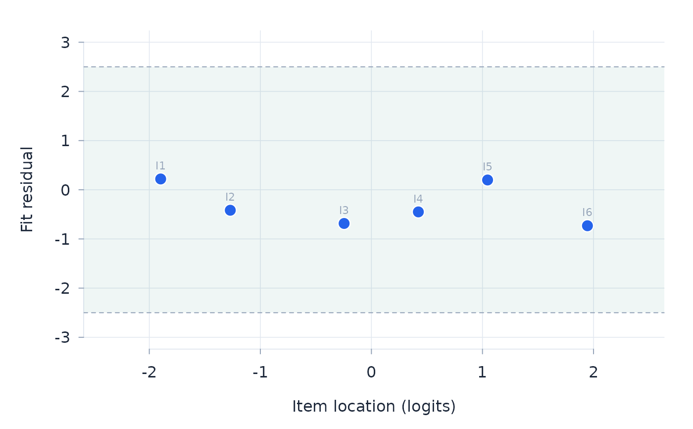
Plot the item map (location against fit residual)

Fitted columns plotted by location and a fit statistic, with the conventional acceptance band at +/- 2.5. The default statistic is the log-of-mean-square fit residual; "infit" and "outfit" display the Wilson–Hilferty standardised mean squares, to which the same band convention applies. MFRM and EFRM points are response cells; ordinary Rasch points are items.

Usage

plot_item_map(fit, statistic = c("residual", "infit", "outfit"), band = 2.5)

Arguments

fit: A fitted object from rasch.
statistic: "residual" (the default fit residual), "infit", or "outfit".
band: Acceptance band for the standardised statistic.

Value

Called for its plotting side effect; invisibly NULL.

Examples

set.seed(1)
d <- seq(-2, 2, length.out = 6)
X <- matrix(rbinom(400 * 6, 1, plogis(outer(rnorm(400), d, "-"))), 400, 6)
colnames(X) <- paste0("I", 1:6)
plot_item_map(rasch(X))