
When to use the MFRM
The many-facet Rasch model (Linacre 1989) extends the Rasch model
(Rasch 1960) to responses jointly indexed by a person, an item, and one
or more measurement facets such as rater, task, or occasion. Use
rasch_mfrm for such designs. A positive facet parameter
denotes greater severity. Person-group variables such as sex or
treatment are not facets: carry them as person factors and assess them
with dif_anova.
For facet levels \(f_1,\ldots,f_Q\), the model is
\[ P(X_{ni\mathbf{f}}=x)= \frac{\exp\left\{x\theta_n- \sum_{k=1}^{x}\left(\delta_{ik}+\sum_{q=1}^{Q}\rho_{qf_q}\right)\right\}} {\sum_{y=0}^{m_i}\exp\left\{y\theta_n- \sum_{k=1}^{y}\left(\delta_{ik}+\sum_{q=1}^{Q}\rho_{qf_q}\right)\right\}}. \]
Item thresholds have a common sum-zero origin, and the levels of each facet sum to zero.
d <- simulate_mfrm(n_persons = 60, n_items = 4, n_raters = 5,
                   rater_severity_sd = 0.7, seed = 8)
person_group <- setNames(rep(c("A", "B"), length.out = 60),
                         unique(d$person))
d$group <- person_group[d$person]
fit <- rasch_mfrm(d, person = "person", item = "item", score = "score",
                  facets = "rater", factors = "group")
fit
#> rasch multiple ratings analysis: 4 items x 5 rater level(s) = 20 response cells, 60 persons
#> Pairwise conditional ML: converged in 7 iterations
#> PSI 0.922, separation quality: excellent
#>
#> Facet 'rater' severities (logits):
#>  level severity    se   n fit_resid
#>     R1    0.800 0.084 240    -0.013
#>     R2    0.567 0.082 240     0.005
#>     R3   -0.992 0.110 240     0.232
#>     R4   -0.503 0.082 240    -0.282
#>     R5    0.128 0.090 240    -0.523
#> (pooled fit residuals and their df on fit$facet_effects)
#>
#> Notes: item I1:R2: category 0 has only 7 response(s); all of the item's jointly estimated thresholds are unreliable at this sparsity (SEs reported as NA) -- consider pc_components or collapsing categories; item I1:R3: only 0 response(s) in category 0; threshold(s) 1 and the item location are weakly determined (SE reported as NA) -- consider pc_components or collapsing categories; item I1:R3: category 0/1 has only 0/3 response(s); all of the item's jointly estimated thresholds are unreliable at this sparsity (SEs reported as NA) -- consider pc_components or collapsing categories; item I1:R4: only 0 response(s) in category 0; threshold(s) 1 and the item location are weakly determined (SE reported as NA) -- consider pc_components or collapsing categories; item I1:R4: category 0/1 has only 0/5 response(s); all of the item's jointly estimated thresholds are unreliable at this sparsity (SEs reported as NA) -- consider pc_components or collapsing categories; item I1:R5: category 0 has only 4 response(s); all of the item's jointly estimated thresholds are unreliable at this sparsity (SEs reported as NA) -- consider pc_components or collapsing categories; item I2:R1: category 3 has only 4 response(s); all of the item's jointly estimated thresholds are unreliable at this sparsity (SEs reported as NA) -- consider pc_components or collapsing categories; item I2:R3: category 0/1 has only 4/7 response(s); all of the item's jointly estimated thresholds are unreliable at this sparsity (SEs reported as NA) -- consider pc_components or collapsing categories; item I3:R1: only 2 response(s) in category 3; threshold(s) 3 and the item location are weakly determined (SE reported as NA) -- consider pc_components or collapsing categories; item I3:R1: category 3 has only 2 response(s); all of the item's jointly estimated thresholds are unreliable at this sparsity (SEs reported as NA) -- consider pc_components or collapsing categories; item I3:R2: category 2/3 has only 7/6 response(s); all of the item's jointly estimated thresholds are unreliable at this sparsity (SEs reported as NA) -- consider pc_components or collapsing categories; item I3:R3: category 0 has only 5 response(s); all of the item's jointly estimated thresholds are unreliable at this sparsity (SEs reported as NA) -- consider pc_components or collapsing categories; item I4:R1: only 0 response(s) in category 3; threshold(s) 3 and the item location are weakly determined (SE reported as NA) -- consider pc_components or collapsing categories; item I4:R1: category 3 has only 0 response(s); all of the item's jointly estimated thresholds are unreliable at this sparsity (SEs reported as NA) -- consider pc_components or collapsing categories; item I4:R2: only 2 response(s) in category 3; threshold(s) 3 and the item location are weakly determined (SE reported as NA) -- consider pc_components or collapsing categories; item I4:R2: category 2/3 has only 5/2 response(s); all of the item's jointly estimated thresholds are unreliable at this sparsity (SEs reported as NA) -- consider pc_components or collapsing categories; item I4:R5: only 2 response(s) in category 3; threshold(s) 3 and the item location are weakly determined (SE reported as NA) -- consider pc_components or collapsing categories; item I4:R5: category 3 has only 2 response(s); all of the item's jointly estimated thresholds are unreliable at this sparsity (SEs reported as NA) -- consider pc_components or collapsing categories; a universal raw-score conversion is not defined across the expanded facet response cells; use the design-specific information curves
Read the structural parameters
The model estimates item thresholds and facet severities together. Internally, each observed item-by-facet combination is a virtual item whose thresholds are the item thresholds shifted by the relevant facet effects. Pairwise conditioning removes the person parameter before calibration.
fit$item_effects
#>  item location    se   n infit_ms outfit_ms fit_resid fit_resid_pooled  df_fit
#>    I1   -1.184 0.092 300    1.038     1.074     0.128            0.777 281.250
#>    I2   -0.411 0.063 300    1.064     1.006     0.031            0.179 281.250
#>    I3    0.464 0.066 300    1.008     1.003    -0.003            0.148 281.250
#>    I4    1.132 0.107 300    0.910     0.859    -0.620           -1.278 281.250
fit$facet_effects$rater
#>  level severity    se   n infit_ms outfit_ms fit_resid fit_resid_pooled df_fit
#>     R1    0.800 0.084 240    1.070     0.993    -0.013            0.064    225
#>     R2    0.567 0.082 240    1.027     0.989     0.005            0.013    225
#>     R3   -0.992 0.110 240    0.959     1.113     0.232            1.007    225
#>     R4   -0.503 0.082 240    1.042     0.942    -0.282           -0.437    225
#>     R5    0.128 0.090 240    0.937     0.889    -0.523           -1.008    225
head(fit$item_thresholds)
#>  item k    tau    se
#>    I1 1 -2.168 0.289
#>    I1 2 -1.348 0.183
#>    I1 3 -0.036 0.156
#>    I2 1 -1.638 0.220
#>    I2 2 -0.456 0.178
#>    I2 3  0.860 0.168
plot_facets(fit, facet = "rater")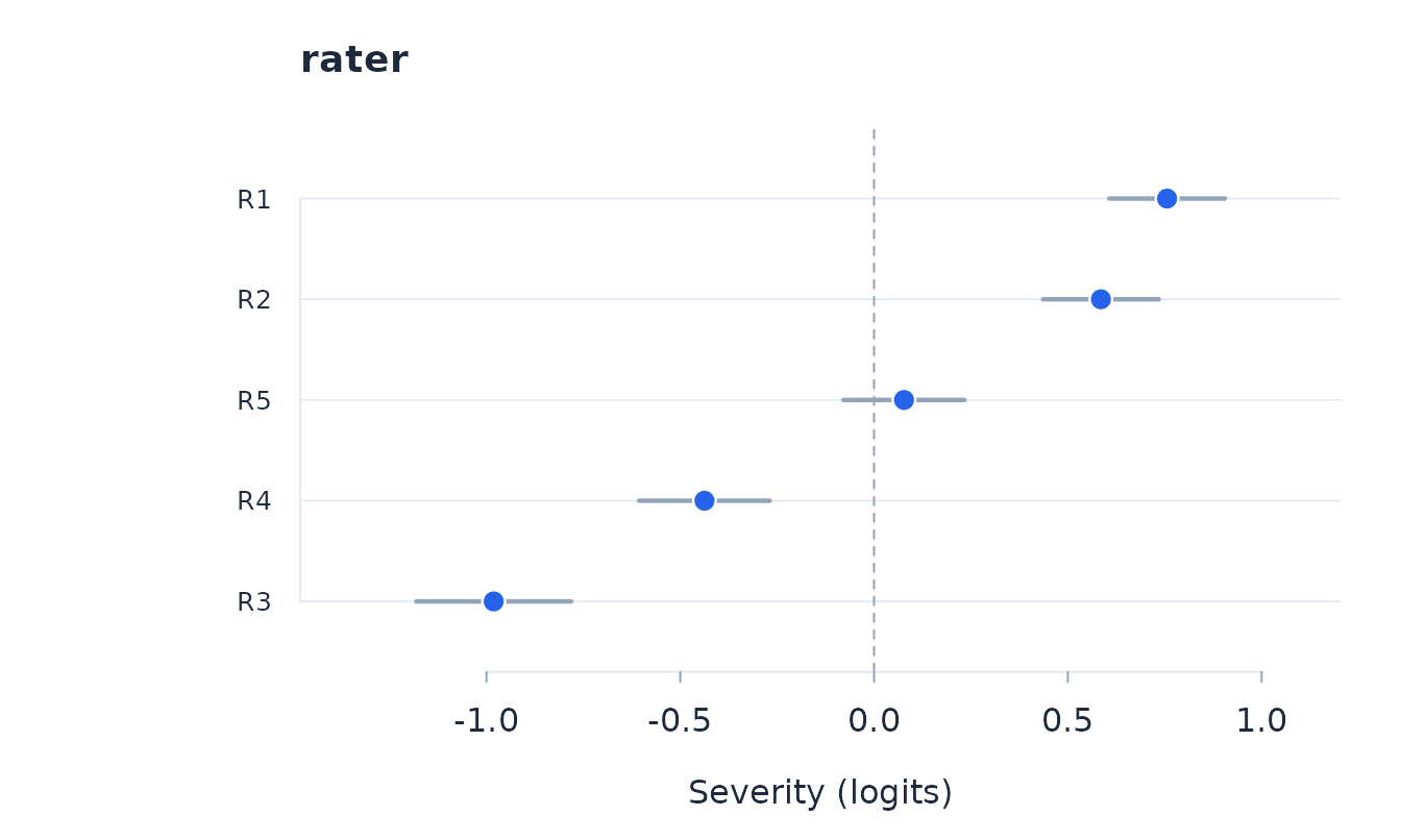
The design must connect facet levels through common items and
persons. A facet nested within an item or a person-disjoint block can be
confounded with item location. rasch_mfrm checks the
structural rank and informative co-observation graph and stops when the
decomposition is not identified.
Item-by-facet interaction
The additive model assumes that severity differences are invariant
across items. When the design and substantive question require it,
interaction adds item-by-level terms with double
sum-to-zero constraints.
fit_interaction <- rasch_mfrm(
  d, person = "person", item = "item", score = "score",
  facets = "rater", interaction = "rater"
)
head(fit_interaction$interaction_effects)
#>  item level  gamma    se      t df     p p_adj significant
#>    I1    R1 -0.119 0.170 -0.698 59 0.488 1.000
#>    I2    R1  0.013 0.128  0.100 59 0.921 1.000
#>    I3    R1  0.031 0.156  0.201 59 0.841 1.000
#>    I4    R1  0.075 0.142  0.526 59 0.601 1.000
#>    I1    R2 -0.015 0.145 -0.103 59 0.918 1.000
#>    I2    R2 -0.083 0.154 -0.539 59 0.592 1.000
fit_interaction$interaction_test
#>  facet df  wald     f df2     p min_effective_persons minimum_required
#>  rater 12 7.684 0.521  48 0.891                    60               30
#>  inference_available
#>                    *
The interaction model retains equal discrimination, but comparisons
among raters become item-dependent. A material interaction therefore
qualifies the claim of invariant rater severity rather than merely
improving fit. The joint Wald test is the primary test of the
interaction family; individual cells are exploratory and adjusted by
Holm’s method. The test uses the least-supported item-by-level cell and
withholds probabilities when that cell has fewer than
max(30, q + 2) persons or effective persons, where
q is the omnibus degrees of freedom.
Diagnostics
The returned object is also a rasch fit in which each
item-by-facet cell enters as its own column of the response matrix (a
virtual item), so the fit, targeting, dependence,
dimensionality, and plotting functions remain available. MFRM margin
tables additionally report an equal-cell fit residual and a
response-weighted pooled residual. Their weighting differs, so both the
design and the location of any misfit should guide interpretation.
Person factors are tested with the ordinary DIF analysis. The optional bootstrap conditions on each person’s total over the observed item-by-facet cells and repeats both the facet calibration and the complete DIF family. Its familywise probabilities refer to the fitted global invariant null.
dif <- dif_anova(fit)
dif_bootstrap(fit, dif, B = 999, seed = 2026)$summary