Plot an object characteristic curve

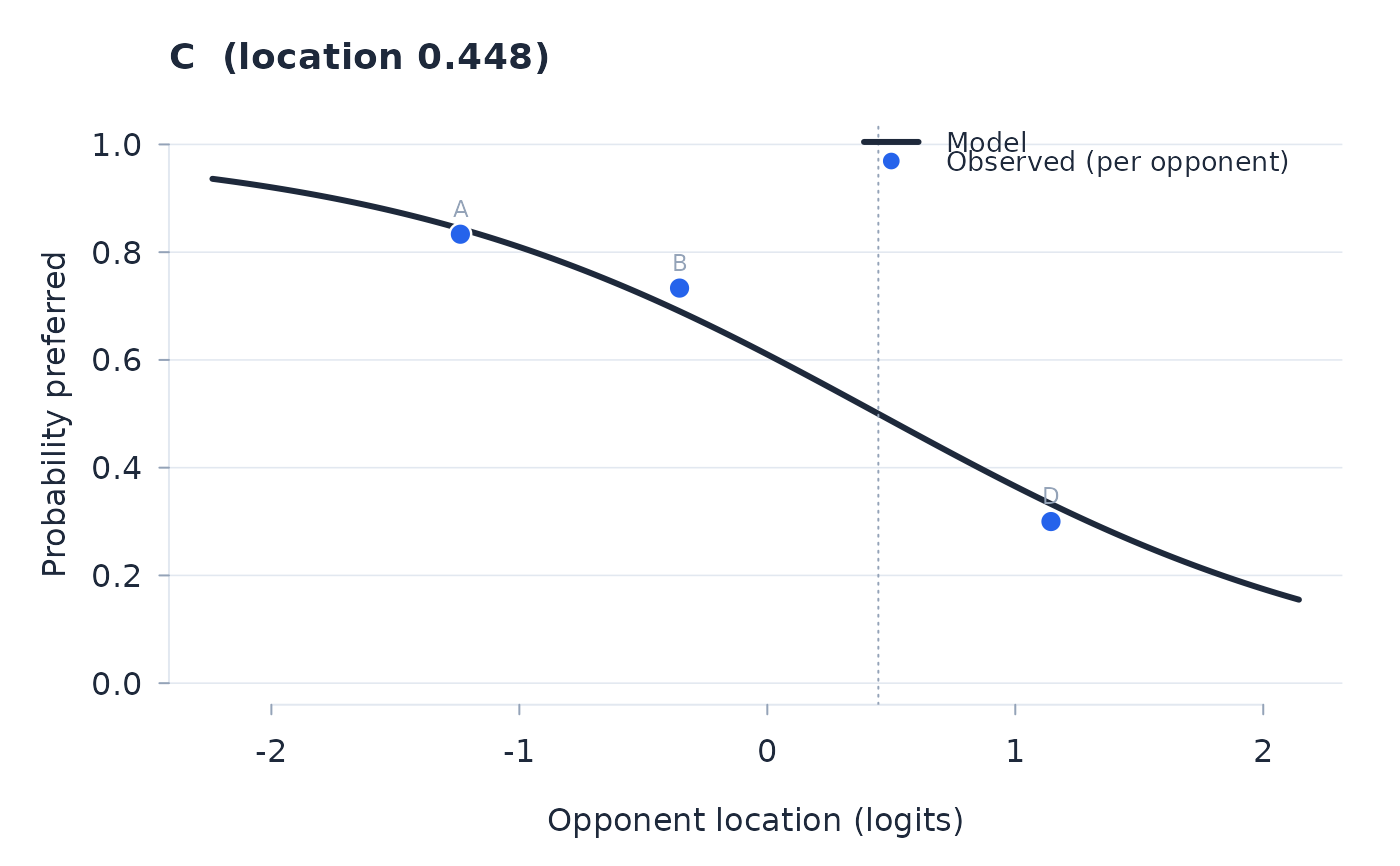
The paired-comparison counterpart of the item characteristic curve: the model expected response for one object as a function of opponent location (the win probability, or the expected graded response), with the observed mean response against each opponent overlaid at that opponent\'s estimated location. Observed points shrink in toward the curve as the model holds; an object of inconsistent quality shows points straying from it, exactly as a misfitting item does.

Usage

plot_btl_icc(fit, object, group = NULL, grid = NULL, min_n = 10)

Arguments

fit

An object from btl.

object

Object name.

group

Optional judge grouping for a DIF overlay: either one value per comparison row of fit$comparisons or a vector named by judge. Observed means are then drawn separately per group, as plot_icc draws person groups.

grid

Opponent-location grid, in logits.

min_n

An opponent's observed point is drawn only when the object (or, in the grouped display, that judge group) met it at least this many times; sparser pairs from incomplete or unbalanced designs are omitted.

Value

Called for its plotting side effect; invisibly the names of the opponents drawn (the ungrouped display), or NULL for the grouped display.

Examples

set.seed(1)
beta <- c(A = -1, B = -0.3, C = 0.4, D = 0.9)
pr <- t(combn(names(beta), 2))
d <- data.frame(a = rep(pr[, 1], each = 30), b = rep(pr[, 2], each = 30))
p <- plogis(beta[d$a] - beta[d$b])
d$win <- ifelse(runif(nrow(d)) < p, d$a, d$b)
plot_btl_icc(btl(d, "a", "b", winner = "win"), "C")