
This vignette follows a Rasch analysis from the overall summary to item and person fit, targeting, dependence, and differential item functioning (DIF). The order matters. A fit statistic is difficult to interpret without knowing whether the scale separates the sample or supplies information over the relevant part of the latent trait.
The same analyses are available in the Shiny application, which follows this same order; the closing section maps each step onto its panel.
The distributed vignette uses precomputed calibration and bootstrap results. The code shown below reproduces them.
Fit the model required by the scoring structure
rasch fits the partial credit model by default (Rasch
1960; Andrich and Marais 2019). Dichotomous data are its one-threshold
special case. Set model = "RSM" only when the same category
threshold structure is intended to hold across items.
For person \(n\), item \(i\), and score \(x=0,\ldots,m_i\), the partial credit model is
\[ P(X_{ni}=x)= \frac{\exp\left\{x\theta_n-\sum_{k=1}^{x}\delta_{ik}\right\}} {\sum_{y=0}^{m_i}\exp\left\{y\theta_n- \sum_{k=1}^{y}\delta_{ik}\right\}}. \]
The rating scale model constrains \(\delta_{ik}=\beta_i+\tau_k\). Pairwise conditioning removes \(\theta_n\) from the item likelihood. Person locations are subsequently estimated by Warm’s weighted likelihood method (Warm 1989).
The example is polytomous and contains three person groups. One item has disordered generating thresholds, one has uniform DIF, and one item pair has local response dependence. These departures make the diagnostic sequence visible without changing the commands used for observed data. Before fitting observed data, check the coding and frequency of every category. Negative scores are read as missing; valid categories begin at zero.
d <- simulate_rasch(
  n_persons = 600,
  n_items = 12,
  model = "PCM",
  n_categories = 4,
  difficulty = c(-1.5, 1.5),
  disordered = "I04",
  dependence = list(pairs = list(c("I10", "I11")), strength = 1.3),
  dif = list(items = "I08", uniform = 0.8),
  n_groups = 3,
  seed = 17
)

fit <- rasch(d, model = "PCM", id = "id", factors = "group")
Overall summary and reliability
The summary establishes whether estimation converged and gives the overall item–trait interaction and reliability. It should be read before individual item or person results.
fit
#> rasch PCM analysis: 12 items, 600 persons
#> Pairwise conditional ML (Zwinderman): converged in 5 iterations
#> PSI 0.851 (no extremes 0.851), item SI 0.995, alpha 0.855, separation quality: good
#> Approximate asymptotic total item-trait chi-square 99.853 on 108 df, p = 0.700
The person separation index (PSI) compares the observed variance of person locations with their mean error variance:
\[ \mathrm{PSI}= \frac{\operatorname{Var}(\hat\theta)- \operatorname{mean}\{\operatorname{SE}(\hat\theta)^2\}} {\operatorname{Var}(\hat\theta)}. \]
The implementation truncates negative values at zero.
fit$psi_noext removes persons with extreme scores and is
useful when extremes inflate the observed spread. The separation ratio
and number of strata express the same information on more interpretable
scales.
The package describes the PSI in broad bands of separation quality. Here the PSI is 0.85, classified as good. This is not the statistical power of a fit test. Fit-test sensitivity also depends on sample size, test length, targeting, category use, trait spread, the test statistic and the departure being tested. Low reliability can weaken the ordering of persons and the formation of class intervals, whereas a large sample can make a small departure statistically significant. Fit residuals, effect sizes, plots and substantive importance remain necessary.
Item estimates, fit, and thresholds
Item locations and their standard errors should be read alongside fit
residuals and the Holm-adjusted item–trait probabilities. The table
shows the six items with the largest absolute residuals; the complete
results are in fit$items. A positive residual indicates
more variation than expected and a negative residual indicates responses
that are more predictable than expected — analytically, the mean squares
behind these residuals compare each item’s empirical
characteristic-curve slope with the average slope, so a negative
residual reads as over-discrimination and a positive one as
under-discrimination (Wu and Adams, 2013). The same source derives the
mean squares’ null variance as roughly \(2/N\), which is why no fixed acceptable
range survives a change of sample size; the conventional \(\pm2.5\) band is a screening rule rather
than a separate hypothesis test, and its meaning moves with \(N\).
item_order <- order(abs(fit$items$fit_resid), decreasing = TRUE)
head(fit$items[item_order, c(
  "item", "location", "se", "fit_resid", "p_adj"
)], 6)
#>  item location    se fit_resid p_adj
#>   I02   -1.244 0.079     1.482 1.000
#>   I07    0.072 0.056     1.477 1.000
#>   I06   -0.147 0.058     1.297 1.000
#>   I01   -1.605 0.106    -1.121 1.000
#>   I05   -0.511 0.059    -0.725 1.000
#>   I09    0.685 0.061    -0.346 1.000
plot_item_map(fit)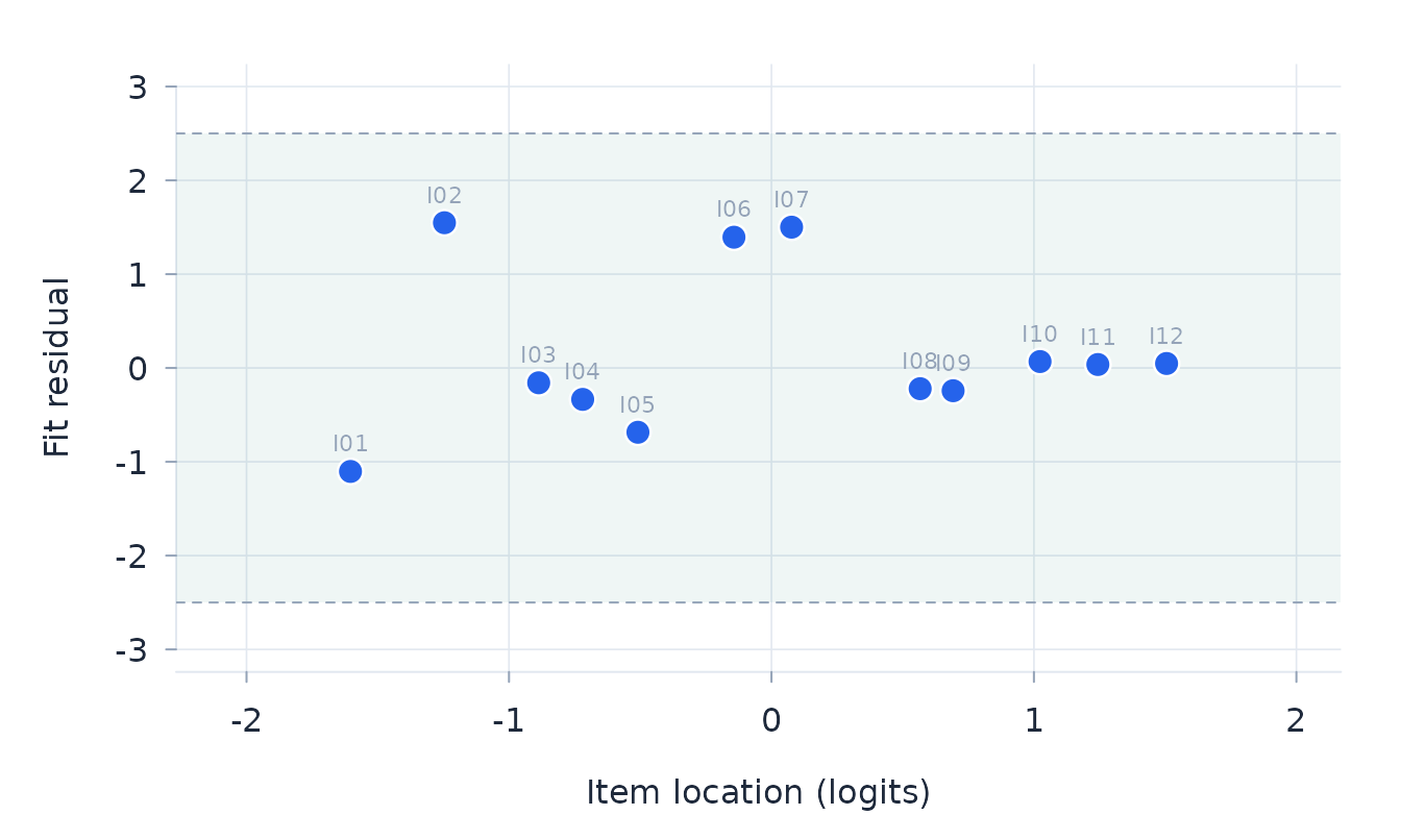
The asymptotic item–trait probabilities treat estimated person
locations as known. fit_bootstrap() instead generates data
under the fitted model and repeats the calibration. The default
conditions on each observed raw score and missingness pattern. Use the
adjusted bootstrap probabilities for item decisions; 999 replicates is a
reasonable minimum for a final analysis, and a larger value may be
needed when there are many items. These references also assume one
independent response row per person. When IDs repeat,
rasch() retains the fit statistics as descriptive summaries
but withholds their probabilities, and fit_bootstrap() is
unavailable. Analyse occasions separately for item-fit inference;
repeated-measures DIF remains available for testing specified occasion
effects. Report B_used, B_nonconverged, and
B_errors. A sparse polytomous calibration may be refused
when too few replicated datasets can be fitted with the same model. For
30 or more requested replicates, inference is withheld unless at least
30 and 90% of the refits are usable. A maxT adjustment is unavailable
for the complete family if one testable member lacks a usable joint
null. Each simulated statistic is standardised against the other
bootstrap rows; using a row in its own reference mean and standard
deviation would make the adjusted probabilities too small. The
adjustment applies separately to each statistic under the fitted global
null. It does not guarantee familywise error among fitting items when
another item misfits. Nominate a primary statistic, or adjust again if
either statistic will be used to make the same confirmatory
decision.
boot <- fit_bootstrap(fit, B = 999, seed = 2026)
head(boot$items[order(boot$items$chisq_p_boot_adj), c(
  "item", "chisq", "chisq_p_boot_adj",
  "fit_resid", "fit_resid_p_boot_adj"
)], 6)
For a polytomous item, successive thresholds should normally increase on the latent scale. The threshold map shows their order directly. Item I04 has an intervening category without its own region on the scale; the category curves show the same problem in probability form.
plot_threshold_map(fit)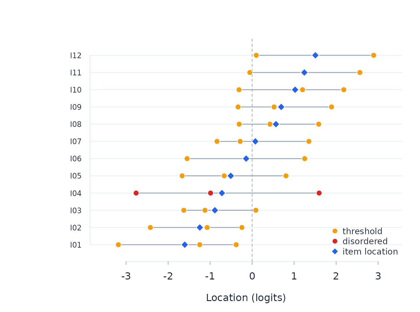
plot_ccc(fit, "I04", observed = TRUE)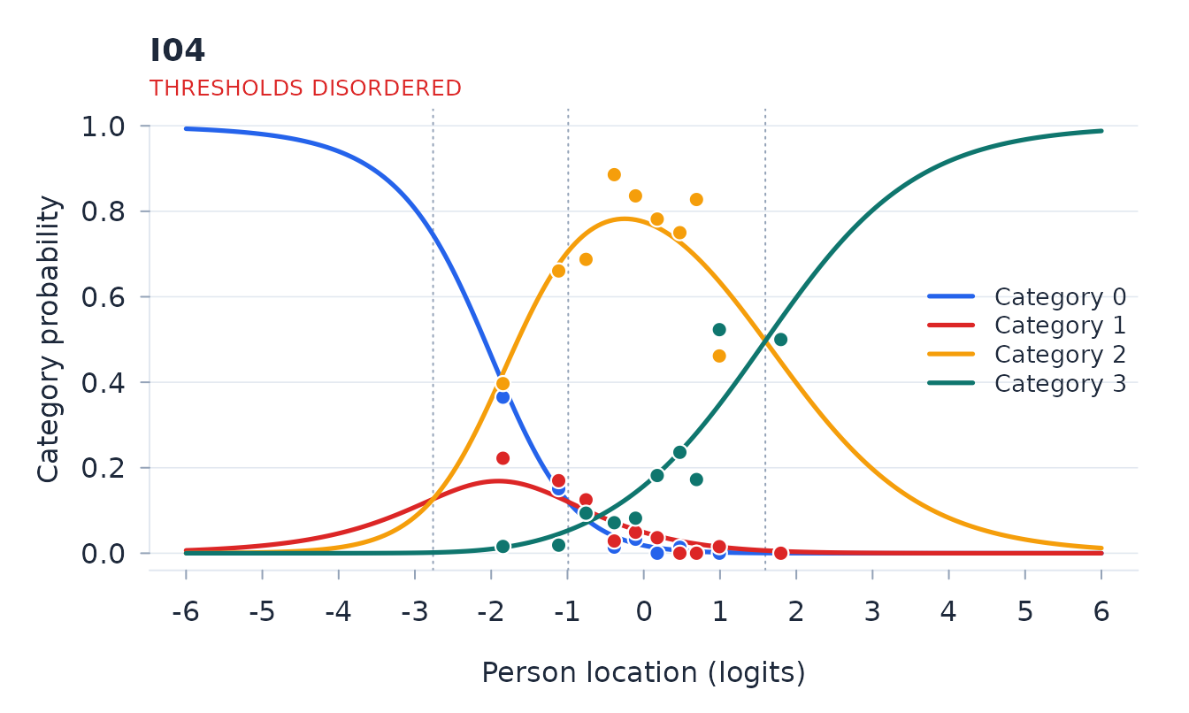
Disordering alone does not justify collapsing categories. The response-option meanings, observed use, and category curves should support any rescoring. The model must then be refitted and checked again.
Person estimates and fit
Person fit addresses the consistency of each response pattern with the fitted scale. The following table puts the largest absolute residuals first. Positive residuals indicate unexpectedly erratic patterns; negative residuals indicate patterns that are unusually predictable.
person_order <- order(abs(fit$person$fit_resid),
                      decreasing = TRUE, na.last = TRUE)
head(fit$person[person_order, c(
  "id", "group", "raw", "theta", "se", "fit_resid"
)], 6)
#>     id group raw  theta    se fit_resid
#>  P0486    g3  18 -0.039 0.377    -3.654
#>  P0001    g1  18 -0.039 0.377    -3.349
#>  P0238    g1  23  0.683 0.393    -3.308
#>  P0031    g1  11 -1.036 0.393     3.051
#>  P0493    g1  21  0.387 0.384    -3.022
#>  P0327    g3  22  0.533 0.388    -2.818
plot_person_fit(fit)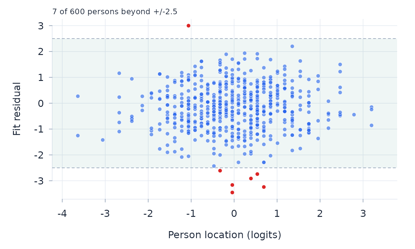
The same score-conditional replicates calibrate person fit without assuming a person distribution. Each person is compared with response patterns having the same raw score and observed items; resampling people would mix different scores and response opportunities. A maximum-statistic reference adjusts the probabilities jointly across persons for each statistic.
head(boot$persons[order(boot$persons$fit_resid_p_boot_adj), c(
  "id", "raw", "theta", "fit_resid", "fit_resid_p_boot_adj"
)], 6)
An unexpected response pattern may reflect coding or data-entry
errors, careless responding, a secondary trait, or a genuine but unusual
person. It is not, by itself, a reason to remove the person. In this
example, 8 persons (1.3%) fall outside the displayed band; the plot
reports the same count and percentage. The statistic
argument displays the standardised infit or outfit in place of the fit
residual, under the same band. Fit residuals are unavailable for extreme
response patterns because those patterns do not provide an interior
location at which fit can be assessed.
Targeting and information
Targeting concerns the match between the person distribution and the item threshold distribution. The table reports their locations and spread, the proportions of persons beyond the threshold range, and the principal reliability indices.
fit$targeting
#> $person_mean
#> [1] -0.0148
#>
#> $person_sd
#> [1] 1.059
#>
#> $person_mean_noext
#> [1] -0.0148
#>
#> $item_mean
#> [1] 0
#>
#> $threshold_range
#> [1] -3.179  2.894
#>
#> $prop_below
#> [1] 0.003333
#>
#> $prop_above
#> [1] 0.005
For a Rasch model, test information is the sum of the conditional response variances:
\[ I(\theta)=\sum_i \operatorname{Var}(X_i\mid\theta), \qquad \operatorname{SE}(\hat\theta)\approx I(\theta)^{-1/2}. \]
The person–item map below places person locations and item thresholds on the same logit scale. The information curve shows where the test is most precise.
plot_pimap(fit, information = TRUE)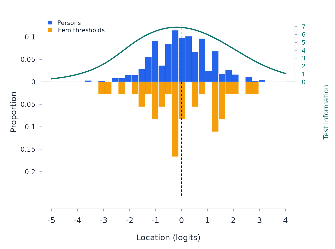
The Wright map shows the same alignment in the conventional vertical arrangement: the person distribution beside the item thresholds on one logit scale.
plot_wright(fit)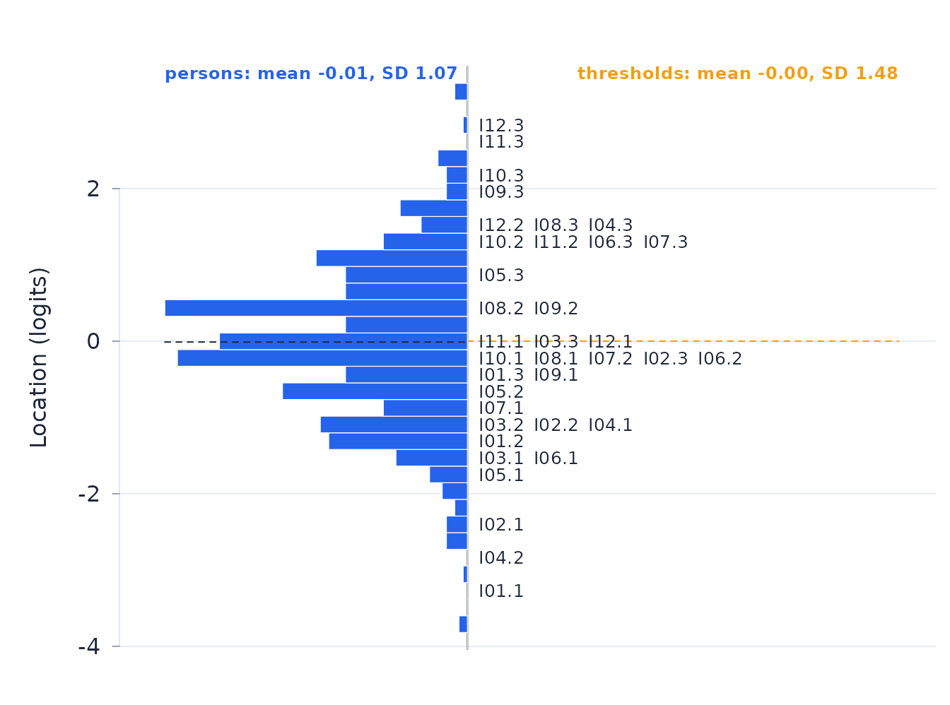
The optional WrightMap package draws the same map with
greater flexibility, including several person and item panels (Torres
Irribarra and Freund 2025). Polytomous thresholds are labelled
t1, t2, and so on. Threshold labels are
omitted for a wholly dichotomous scale; a dichotomous item in a mixed
scale retains t1. Panels should answer a substantive
question; here the person distributions are separated by the fitted
group factor.
if (requireNamespace("WrightMap", quietly = TRUE)) {
  wright_map(fit, person_panels = "group")
}
If WrightMap is not installed, install it with
install.packages("WrightMap") before running this
chunk.
Local and trait dependence
Local response dependence occurs when two responses remain associated
after conditioning on the latent trait. Yen’s \(Q3\) is the correlation between two items’
standardised residuals. Because raw \(Q3\) values have a negative baseline in a
finite test, q3_star subtracts the average off-diagonal
value.
q3 <- residual_correlations(fit)
q3$average
#> [1] -0.0866
head(q3$pairs[, c("item_a", "item_b", "q3", "q3_star")], 5)
#>   item_a item_b        q3 q3_star
#> 1    I10    I11  0.134107 0.22071
#> 2    I02    I05  0.003793 0.09039
#> 3    I01    I04 -0.014196 0.07241
#> 4    I06    I07 -0.016938 0.06966
#> 5    I04    I12 -0.020358 0.06624
plot_resid_cor(fit)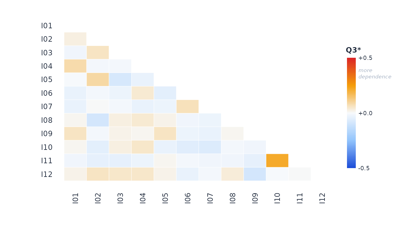
There is no universal critical value for adjusted \(Q3\) (Christensen, Makransky and Horton
2017). Its size, the response process, and the content of the item pair
matter. When theory supports treating dependent items as one superitem,
combine_items() refits the complete calibration and
spread_test() compares its threshold spread with the
binomial bound. The bound does not apply to a superitem containing a
polytomous component.
Trait dependence is examined through the residual components and by comparing person estimates from opposed item subsets (Smith 2002). For subsets \(A\) and \(B\), the person-level statistic is
\[ t_n=\frac{\hat\theta_{nA}-\hat\theta_{nB}} {\sqrt{\operatorname{SE}(\hat\theta_{nA})^2+ \operatorname{SE}(\hat\theta_{nB})^2}}. \]
The observed proportion, binomial interval and score points describe the comparison. Unequal targeting can shift the per-person null rate even for subsets fixed in advance. A dimensionality verdict therefore uses a parametric bootstrap, retaining a fixed split or repeating the selection when the split comes from the residuals.
dimensionality <- dimensionality_test(
  fit,
  items_positive = paste0("I", sprintf("%02d", 1:6)),
  items_negative = paste0("I", sprintf("%02d", 7:12)),
  B = 199, seed = 2026
)
scree <- plot_scree(fit, seed = 2026)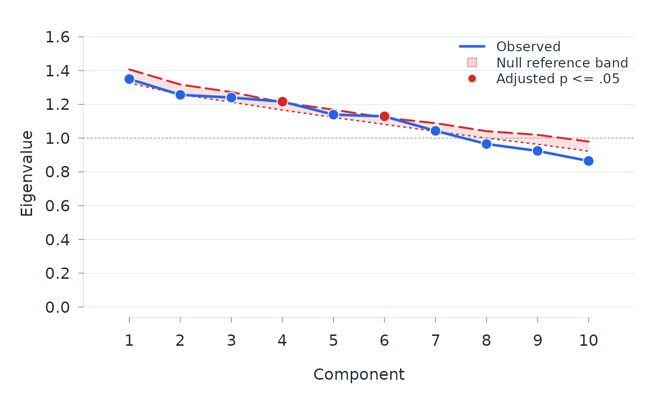
The band shows the residual eigenvalues expected under the fitted model. Red points clear its familywise 5% limit; the returned table contains both raw and adjusted simulation probabilities.
plot_pca(fit)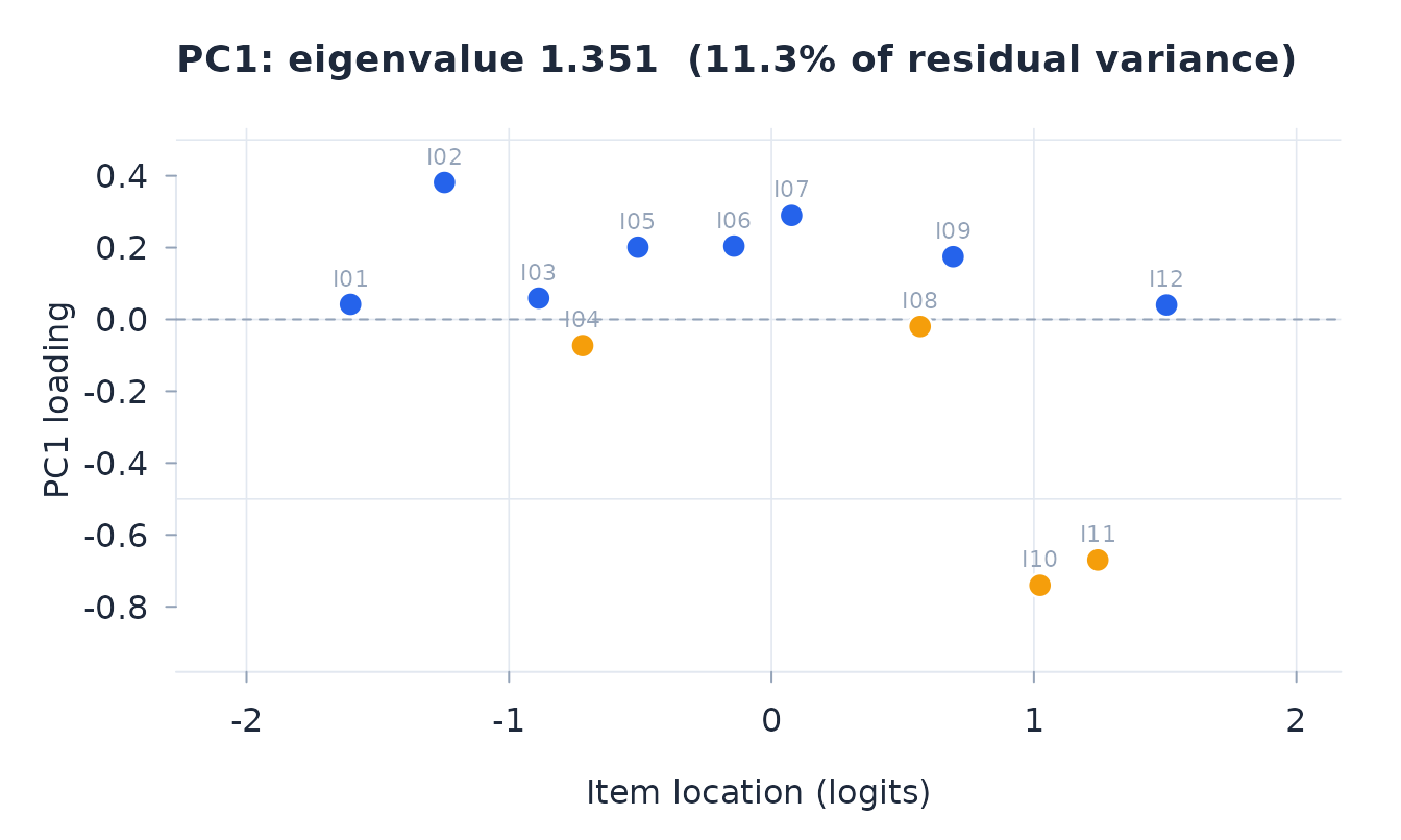
Here, 3.0% of the person comparisons are significant (Clopper–Pearson 95% interval 1.8% to 4.8%). The bootstrap probability is 0.655. The smaller subset contains 18 score points. A quiet result from a short subtest is inconclusive rather than evidence that a secondary trait is absent.
Differential item functioning
Person factors must be nominated when the model is fitted. With a person factor \(G\) and trait class interval \(C\), the residual model is
\[ z=\mu+G+C+G\mathbin{:}C+\varepsilon. \]
The factor term tests uniform DIF; the interaction with class
interval tests non-uniform DIF. dif_anova() fits all
nominated factors together, recognises within-person factors in repeated
designs, and applies Holm familywise correction over the item-by-term
tests.
dif <- dif_anova(fit, sizes = TRUE)
flagged_dif <- subset(dif$summary, uniform_DIF | nonuniform_DIF)
flagged_dif[, c(
  "item", "term", "F_uniform", "p_uniform_adj", "eta2_uniform",
  "F_nonuniform", "p_nonuniform_adj", "eta2_nonuniform"
)]
#>  item  term F_uniform p_uniform_adj eta2_uniform F_nonuniform p_nonuniform_adj
#>   I08 group    20.993       < 0.001        0.069        1.220            1.000
#>  eta2_nonuniform
#>            0.021
plot_icc(fit, "I08", group = "group")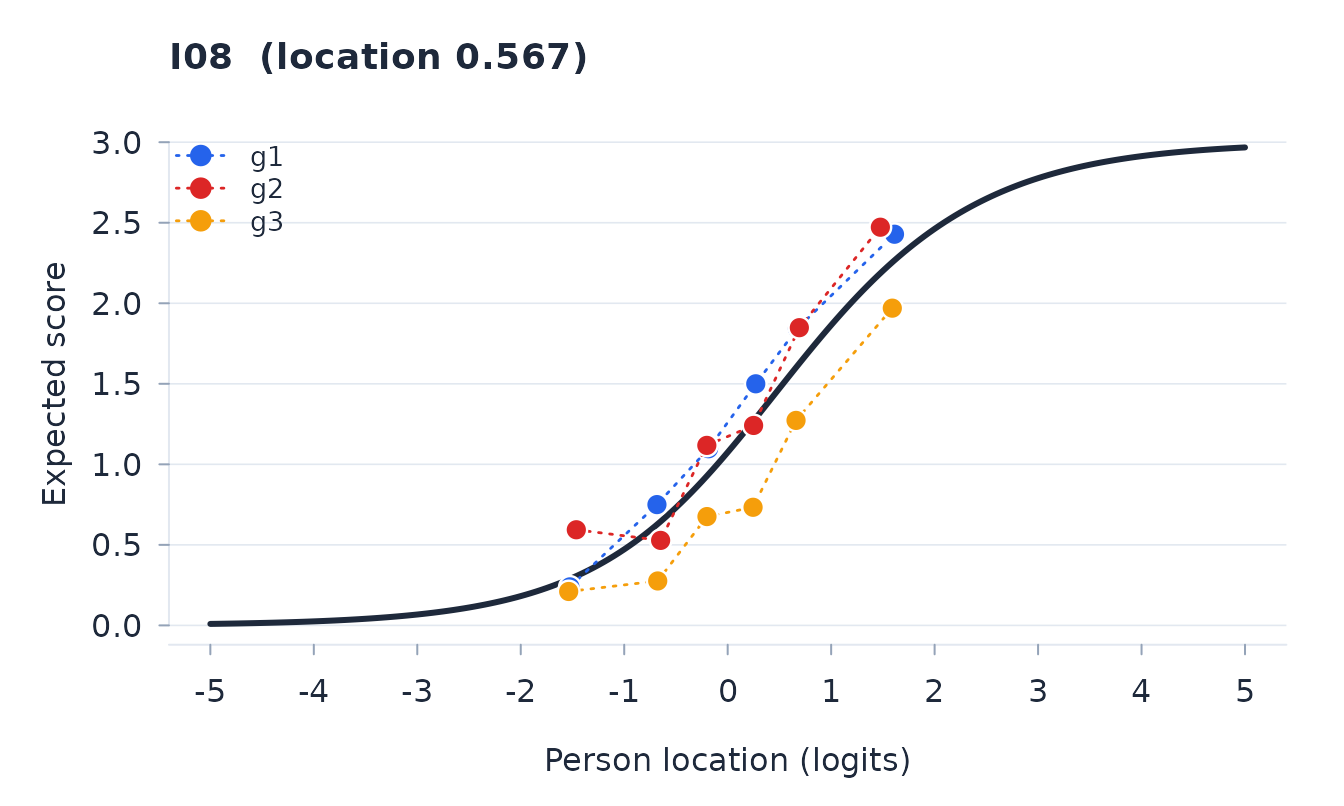
For a significant factor with more than two levels, the follow-up
should estimate the relevant differences in Rasch logits rather than
rely on a generic Tukey procedure. With sizes = TRUE,
dif_anova() returns the Holm-adjusted marginal pairwise
comparisons for significant main effects and difference-in-differences
for significant interactions.
dif$posthoc[, c(
  "item", "contrast", "estimate", "se", "p_adj",
  "lower", "upper", "practical"
)]
#>  item contrast estimate    se   p_adj  lower upper practical
#>   I08  g2 - g1   -0.033 0.138   0.813 -0.304 0.238
#>   I08  g3 - g1    0.711 0.148 < 0.001  0.421 1.001         *
#>   I08  g3 - g2    0.744 0.147 < 0.001  0.457 1.031         *
The residual ANOVA is the primary DIF analysis. A bootstrap sensitivity analysis repeats the calibration and complete DIF analysis under the fitted invariant model. Here it conditions on each person’s score and observed-item pattern; Multiple Ratings and explanatory models use the same sufficient-score principle, Extended Frames conditions within item sets, and Comparative Judgement draws from its fitted outcome model. Its minimum-p probabilities calibrate the same item- or object-by-term family under the fitted global invariant null. They do not guarantee strong familywise control after one member departs. The bootstrap is not a way to purify a scale after DIF has already contaminated the person scores, so disagreement calls for closer review rather than an automatic split.
dif_boot <- dif_bootstrap(fit, dif, B = 999, workers = 4, seed = 2026)
dif_boot$summary[, c(
  "item", "term", "p_uniform_boot_adj", "p_nonuniform_boot_adj"
)]
Statistical significance and practical magnitude answer different
questions. Any split must be supported by the response process and
should be applied with resolve_dif(), which refits the
calibration and updates the item and person estimates. The revised fit
then goes through the same summary, fit, targeting, dependence, and DIF
sequence.
The same analysis in the application
rasch::run_app() runs the sequence above, one panel per
step, and every result carries the call that produced it. The
walkthrough below follows the same order as the code, so a reader can
move between the two.
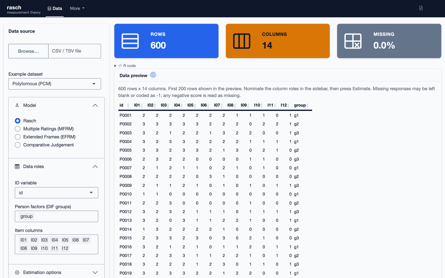
Data imports the responses and assigns each column
its measurement role: person identifier, items, and person factors. The
model is chosen here, and the scoring structure governs that choice
exactly as it does in rasch(). The example datasets in the
sidebar load a complete design with its roles already assigned, which is
the quickest way to see the whole sequence.
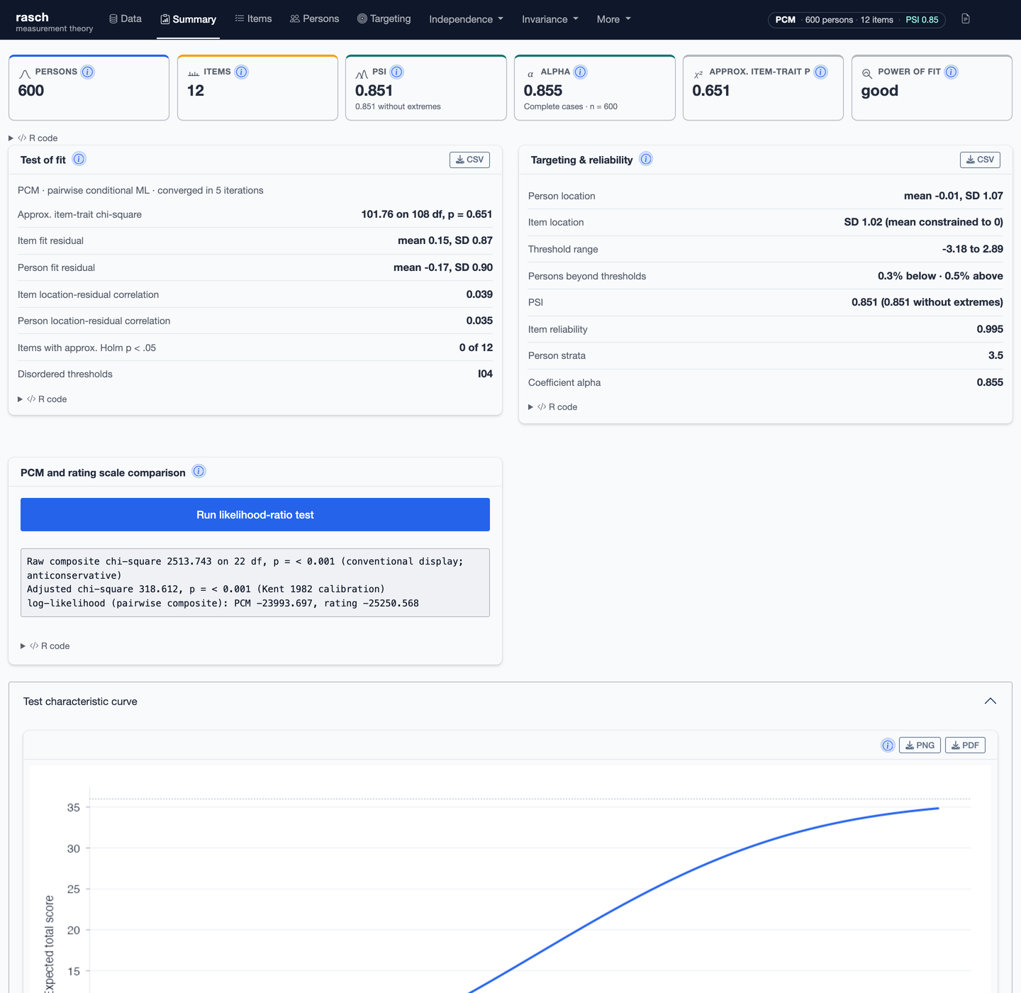
Summary is read first: convergence, the item–trait
interaction, the person separation index and coefficient alpha, and the
targeting of the person distribution against the threshold distribution.
It answers the same questions as fit_summary_table() and
targeting_table() above. Tiles that report a check are
green when it passes and red when it wants attention; tiles that report
a count are coloured by the side of the model they describe, persons
blue and items amber, the colours the Wright and person-item maps
use.
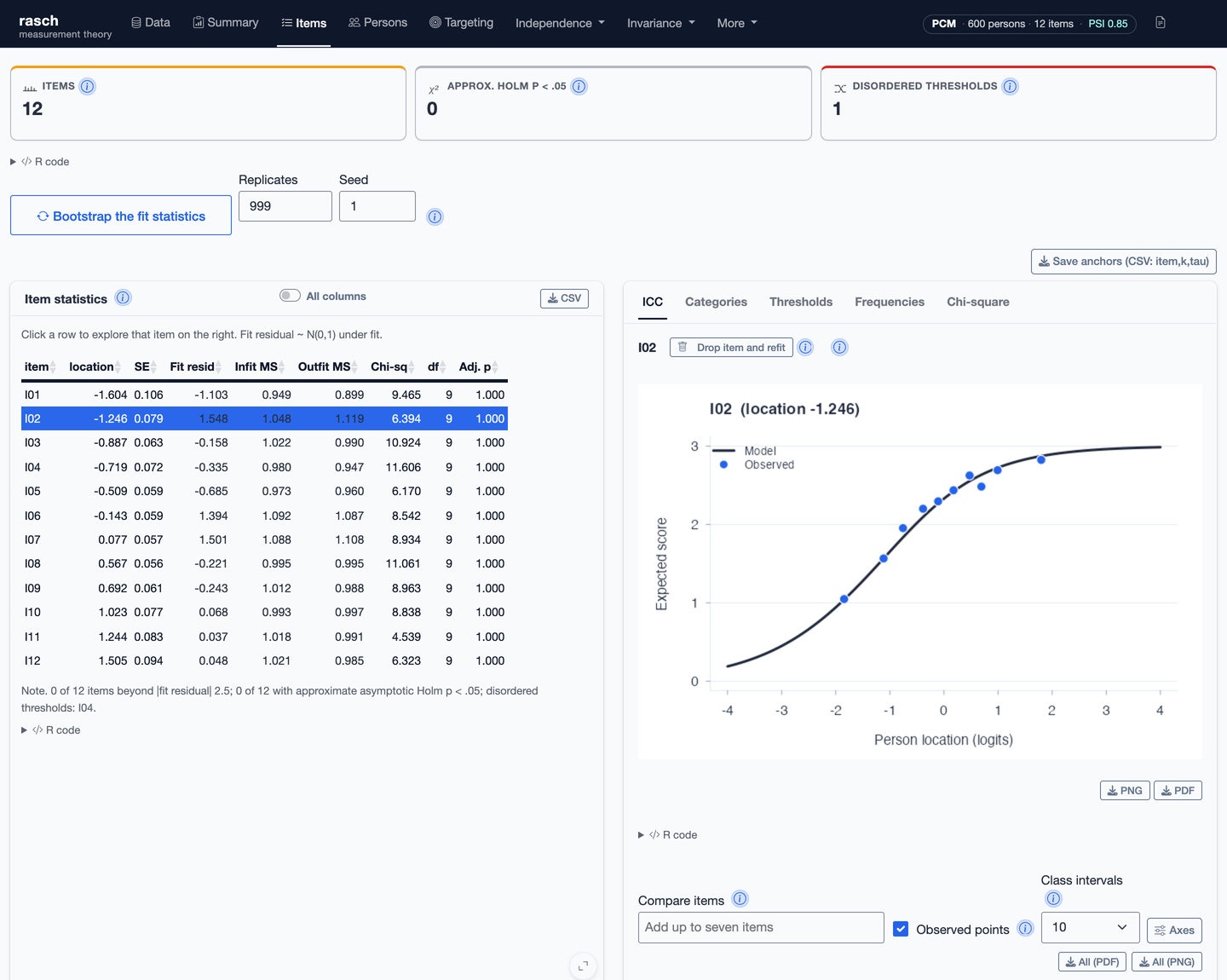
Items carries the estimates and fit statistics of the item table above. Selecting a row draws that item on the right, with tabs for the characteristic curve, the category probabilities, the thresholds, the category frequencies, and the class-interval chi-square. The panels beneath hold the threshold map, the item fit map, the fit residual distribution and the traditional statistics; they open on demand rather than by default. The fit-bootstrap button runs the item and person calibration in the background. Its adjusted probabilities then replace the asymptotic screening probability in the item display and appear in the person table. The run can be cancelled.
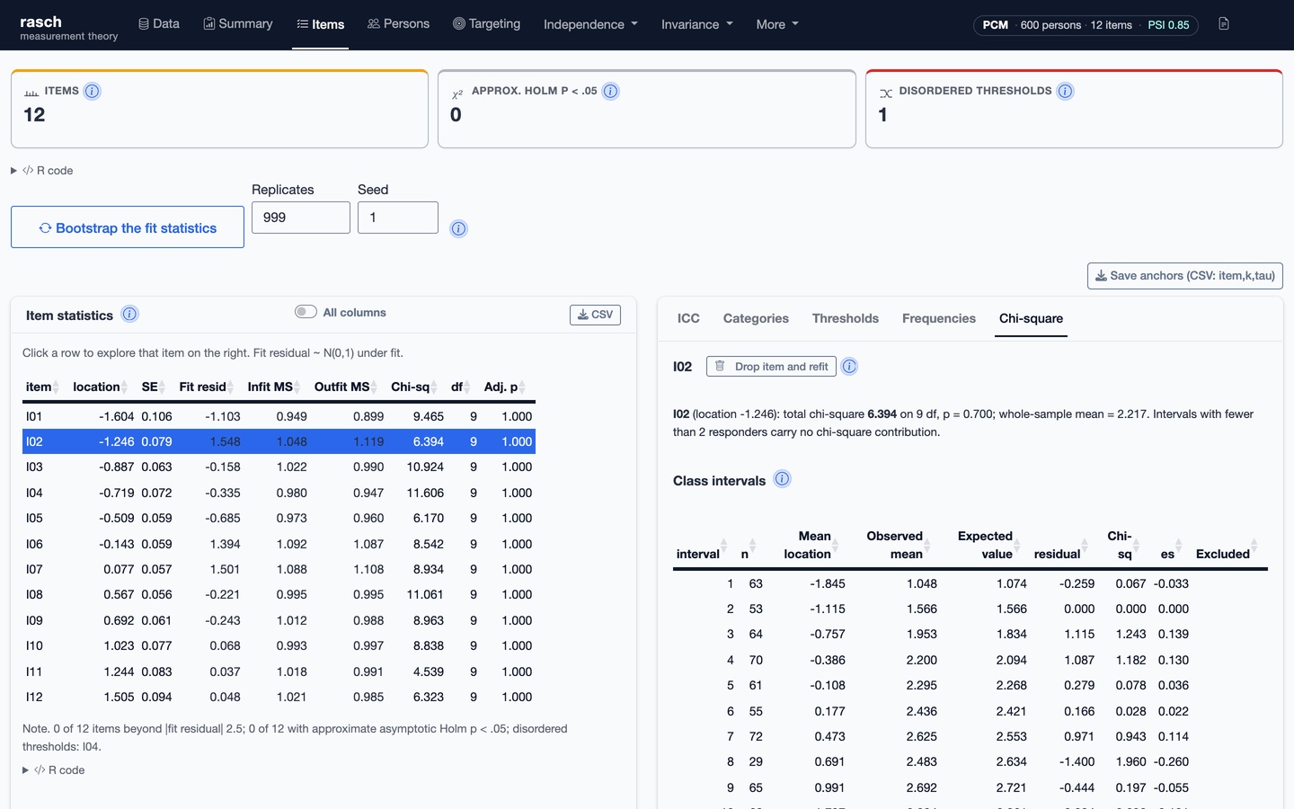
The Chi-square tab is the class-interval breakdown
chisq_detail() returns: per interval the size, the observed
and expected means, the standardised residual and its chi-square
component. It is where a significant item–trait interaction is read as a
pattern rather than a number.
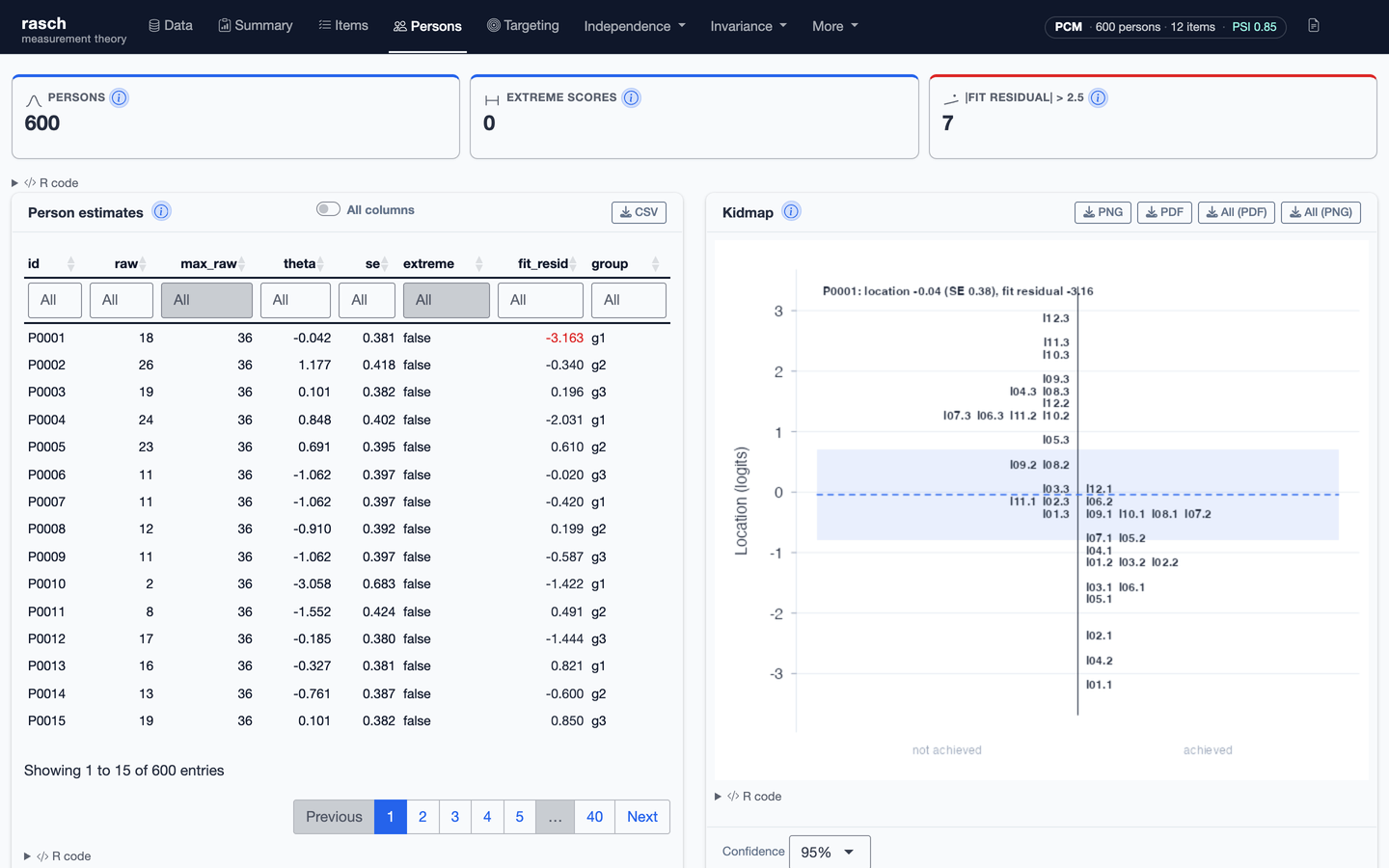
Persons holds the person estimates and their fit,
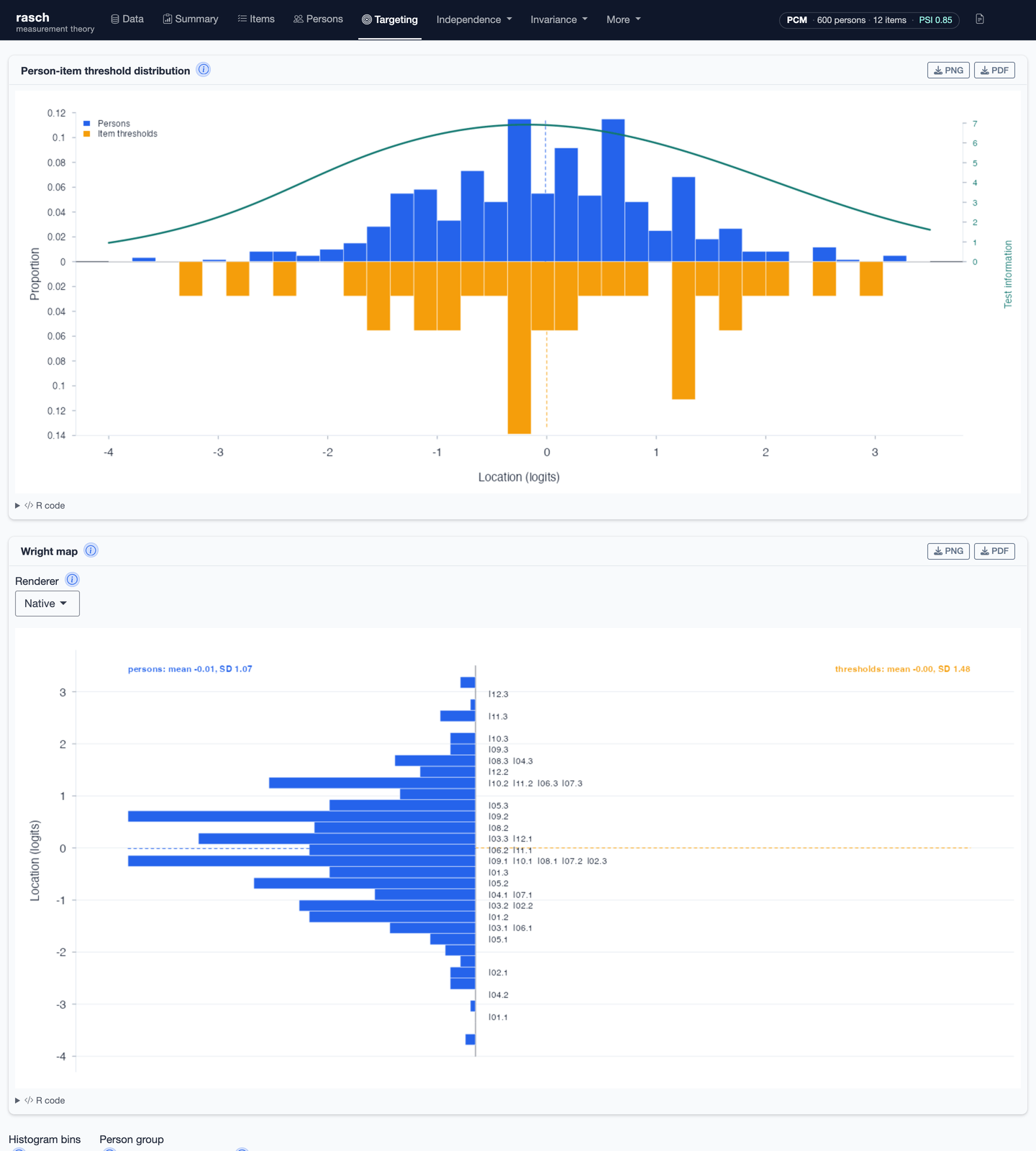
and Targeting the person-item map and the test
information the code produces with plot_pimap() and
test_information(). Both maps can be restricted to one
person group or one item set, and the restriction is named in the legend
so a partial map cannot be read as the whole instrument.
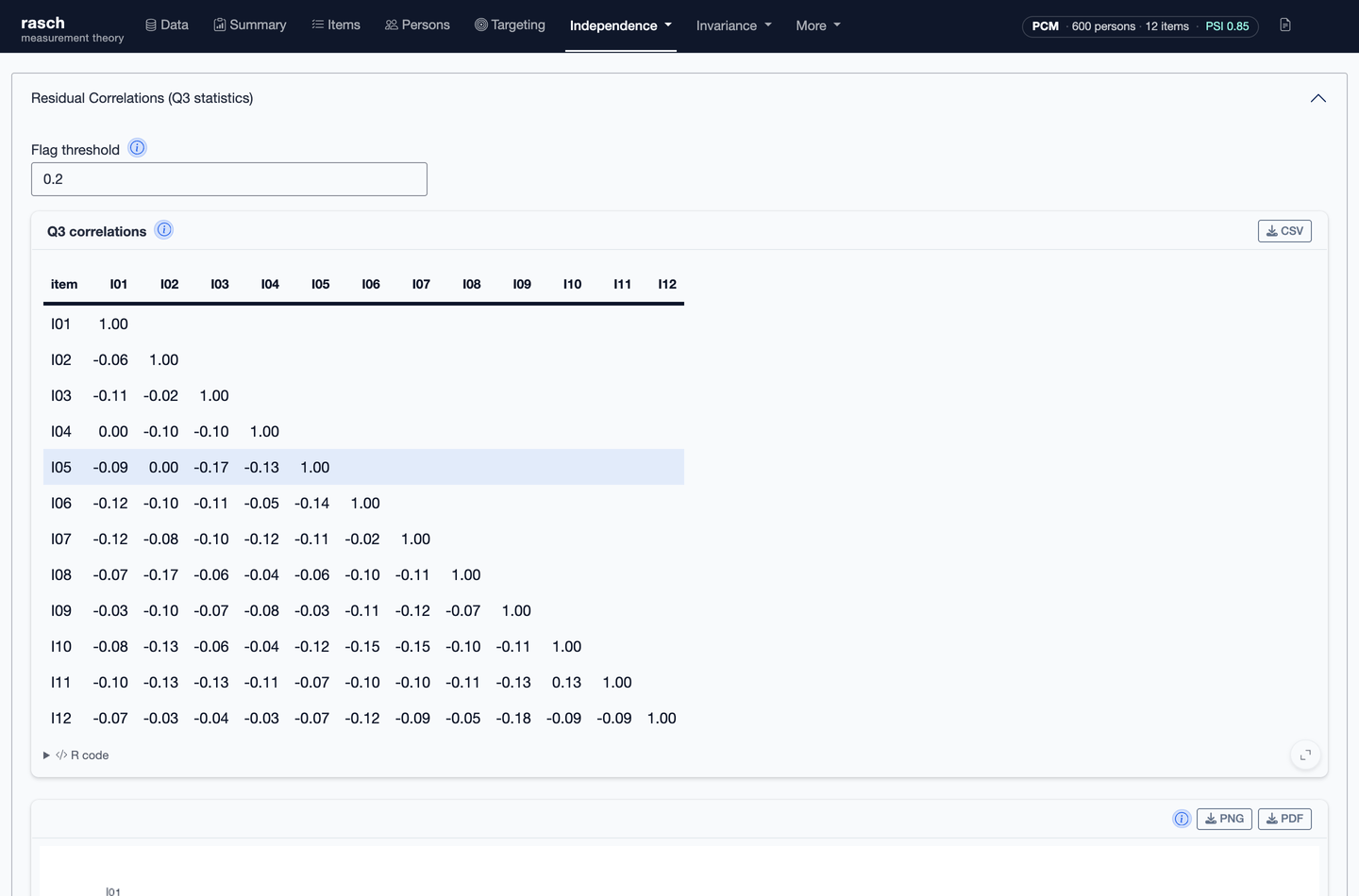
The remaining analyses sit under two menus that divide them by the assumption they examine. Independence holds local dependence and trait dimensionality — the residual correlations and principal components of this vignette’s dependence section. For the person-subset test, choose the same item subsets as above and set Bootstrap replicates to 199 and Random seed to 2026. With zero replicates, the app reports the comparisons descriptively, without a verdict.
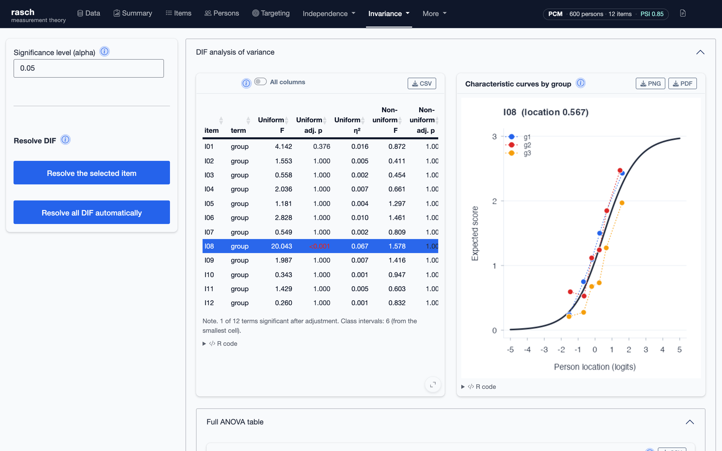
Invariance holds differential item functioning,
equating, guessing, facets and extended frames. The DIF panel runs
dif_anova() over the nominated person factors, reports the
uniform and non-uniform tests with their Holm adjustment and effect
sizes, and draws the observed and expected curves by group for a
selected item. Its bootstrap panel runs the optional sensitivity
analysis in the background and keeps it with saved analyses and
reports.
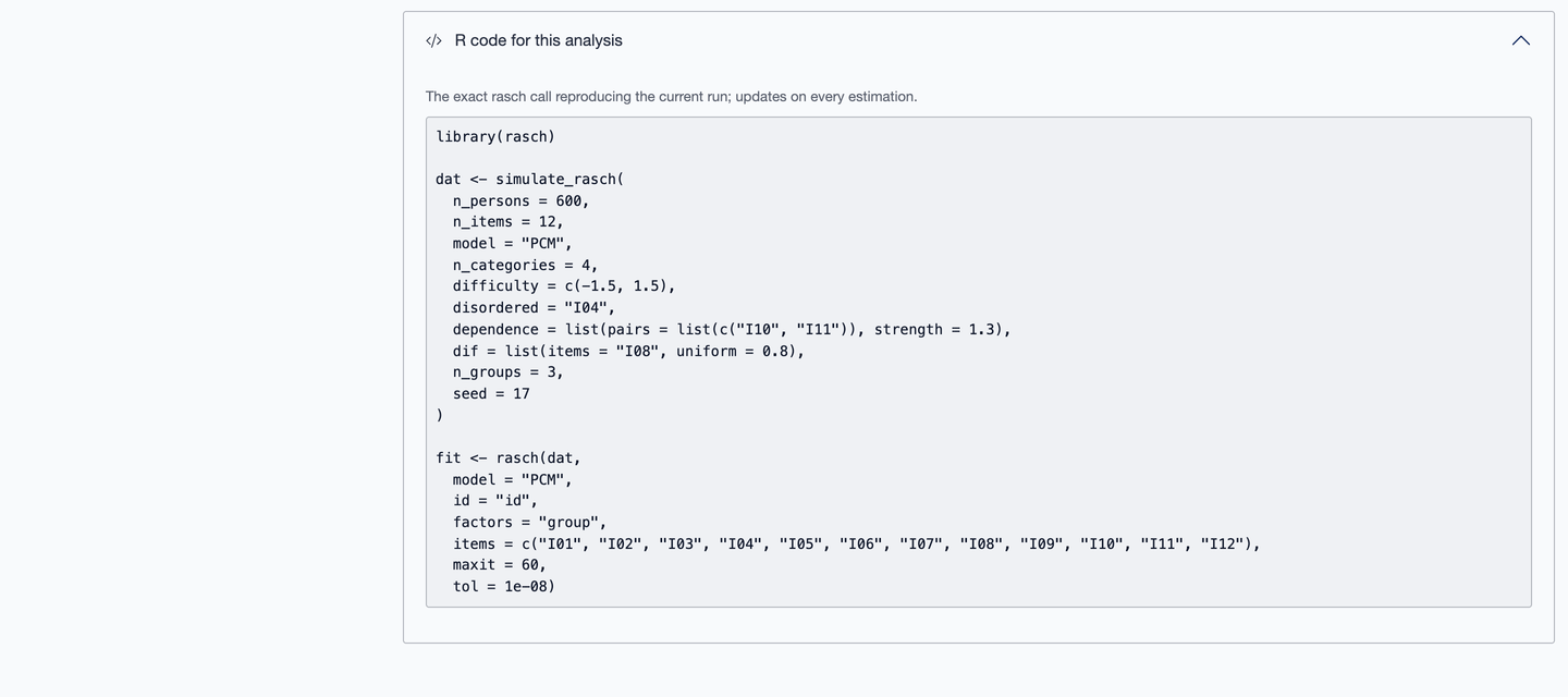
Every result carries an R code disclosure beneath it. Opening it shows the call that produced that table or figure, so an analysis assembled in the application can be read as, and continued as, the script this vignette writes by hand.
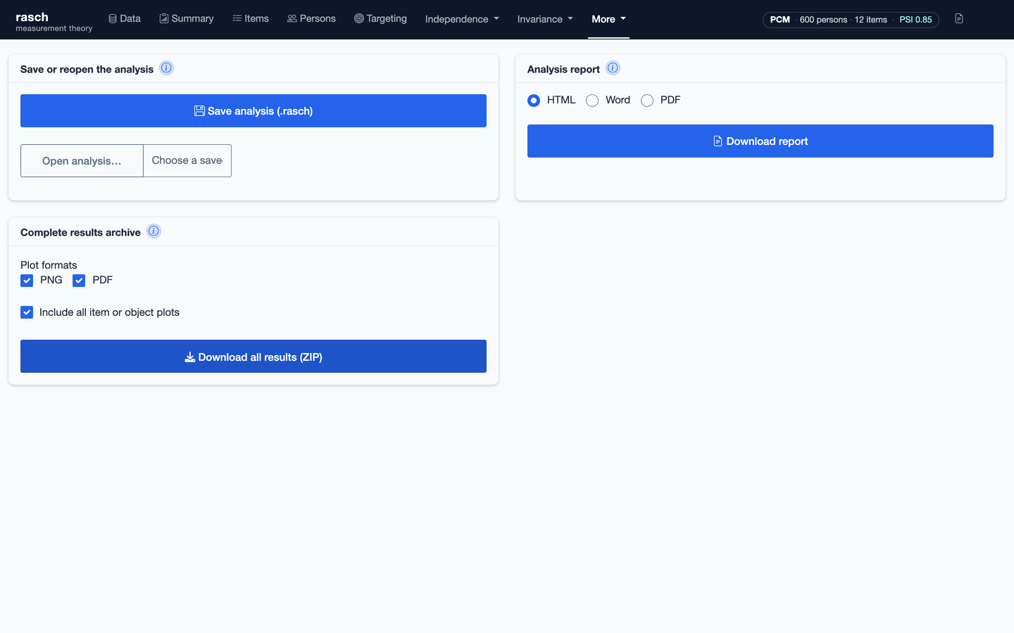
Under More, an analysis can be saved as a
.rasch project and reopened with its data roles and
estimation settings intact, or exported as tables, figures and a
Markdown, Word or PDF report. The same menu holds the simulation designs
of the plant-and-detect vignette and the model comparison that
compare_fits() and lr_test() produce.
Older projects are checked against the current person-scoring
algorithm. If their scores differ, the app asks for a refit and leaves
the original file unchanged. The source data remain accessible with
readRDS(file)$data. Superseded DIF results are omitted with
a warning; rerun those analyses before reporting them.
References
Andrich, D., and Marais, I. (2019). A Course in Rasch Measurement Theory: Measuring in the Educational, Social and Health Sciences. Springer.
Christensen, K. B., Makransky, G., and Horton, M. (2017). Critical values for Yen’s Q3: Identification of local dependence in the Rasch model using residual correlations. Applied Psychological Measurement, 41(3), 178–194.
Holm, S. (1979). A simple sequentially rejective multiple test procedure. Scandinavian Journal of Statistics, 6(2), 65–70.
Molenaar, I. W., and Hoijtink, H. (1996). Person-fit test statistics for the Rasch model. Applied Measurement in Education, 9(1), 87–106.
Rasch, G. (1960). Probabilistic Models for Some Intelligence and Attainment Tests. Copenhagen: Danish Institute for Educational Research. (Expanded edition, 1980, Chicago: University of Chicago Press.)
Smith, E. V. Jr. (2002). Detecting and evaluating the impact of multidimensionality using item fit statistics and principal component analysis of residuals. Journal of Applied Measurement, 3(2), 205–231.
Torres Irribarra, D., and Freund, R. (2025). WrightMap: IRT item-person map with ConQuest integration. R package version 1.5.
Warm, T. A. (1989). Weighted likelihood estimation of ability in item response theory. Psychometrika, 54(3), 427–450.
Wu, M., and Adams, R. J. (2013). Properties of Rasch residual fit statistics. Journal of Applied Measurement, 14(4), 339–355.
Westfall, P. H., and Young, S. S. (1993). Resampling-Based Multiple Testing. Wiley.
Yen, W. M. (1984). Effects of local item dependence on the fit and equating performance of the three-parameter logistic model. Applied Psychological Measurement, 8(2), 125–145.